Chapter 4. Examples

A prior model consisting of three independent 1D distributions (a Gaussian, Laplace, and Uniform distribution) can be defined using

ip=1;
prior{ip}.type='GAUSSIAN';
prior{ip}.name='Gaussian';
prior{ip}.m0=10;
prior{ip}.std=2;

ip=2;
prior{ip}.type='GAUSSIAN';
prior{ip}.name='Laplace';
prior{ip}.m0=10;
prior{ip}.std=2;
prior{ip}.norm=1;

ip=3;
prior{ip}.type='GAUSSIAN';
prior{ip}.name='Uniform';
prior{ip}.m0=10;
prior{ip}.std=2;
prior{ip}.norm=60;

m=sippi_prior(prior);

m = 

    [14.3082]    [9.4436]    [10.8294]

1D histograms of a sample (consisting of 1000 realizations) of the prior models can be visualized using ...

sippi_plot_prior_sample(prior);

The FFT-MA type a priori model allow separation of properties of the covariance model (covariance parameters, such as range, and anisotropy ratio) and the random component of a Gaussian model. This allow one to define a Gaussian a priori model, where the covariance parameters can be treated as unknown variables.

In order to treat the covariance parameters as unknowns, one must define one a priori model of type FFTMA, and then a number of 1D GAUSSIAN type a priori models, one for each covariance parameter. Each gaussian type prior model must have a descriptive name, corresponding to the covariance parameter that is should describe:

prior{im}.type='gaussian';
prior{im}.name='m_0';     % to define a prior for the mean 
prior{im}.name='sill';    % to define a prior for sill (variance)
prior{im}.name='range_1'; % to define a prior for the range parameter 1
prior{im}.name='range_2'; % to define a prior for the range parameter 2
prior{im}.name='range_3'; % to define a prior for the range parameter 3
prior{im}.name='ang_1';   % to define a prior for the first angle of rotation
prior{im}.name='ang_2';   % to define a prior for the second angle of rotation
prior{im}.name='ang_3';   % to define a prior for the third angle of rotation
prior{im}.name='nu';      % to define a prior for the shape parameter, nu 
			  %   (only applies when the Matern type Covariance model is used)

A very simple example of a prior model defining a 1D Spherical type covariance model with a range between 5 and 15 meters, can be defined using:

im=1; 
prior{im}.type='FFTMA';
prior{im}.x=[0:.1:10]; % X array 
prior{im}.m0=10;
prior{im}.Va='1 Sph(10)';
prior{im}.fftma_options.constant_C=0;


im=2;
prior{im}.type='gaussian';
prior{im}.name='range_1';
prior{im}.m0=10;
prior{im}.std=5
prior{im}.norm=80;
prior{im}.prior_master=1; % -- NOTE, set this to the FFT-MA type prior for which this prior type
                          % should describe the range

Note that the the field prior_master must be set to point the to the FFT-MA type a priori model (through its id/number) for which it should define a covariance parameter (in this case the range).

10 independent realizations of this type of a priori model are shown in the following figure

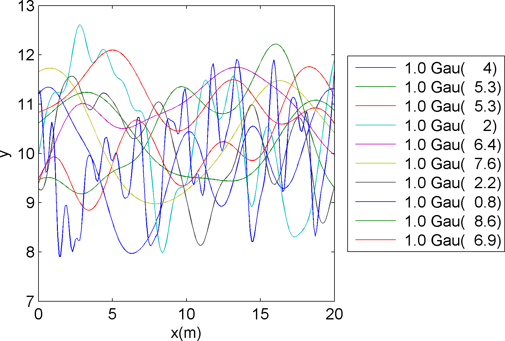Such a prior, as all prior models available in SIPPI, works with sequential Gibbs sampling, allowing a random walk in the space of a prior acceptable models, that will sample the prior model. An example of such a random walk can be performed using

prior{1}.seq_gibbs.step=.005;
prior{2}.seq_gibbs.step=0.1;
clear m_real;
for i=1:150;
    [m,prior]=sippi_prior(prior,m);
    m_real(:,i)=m{1};
end

An example of such a set of 150 dependent realization of the prior can be seen below
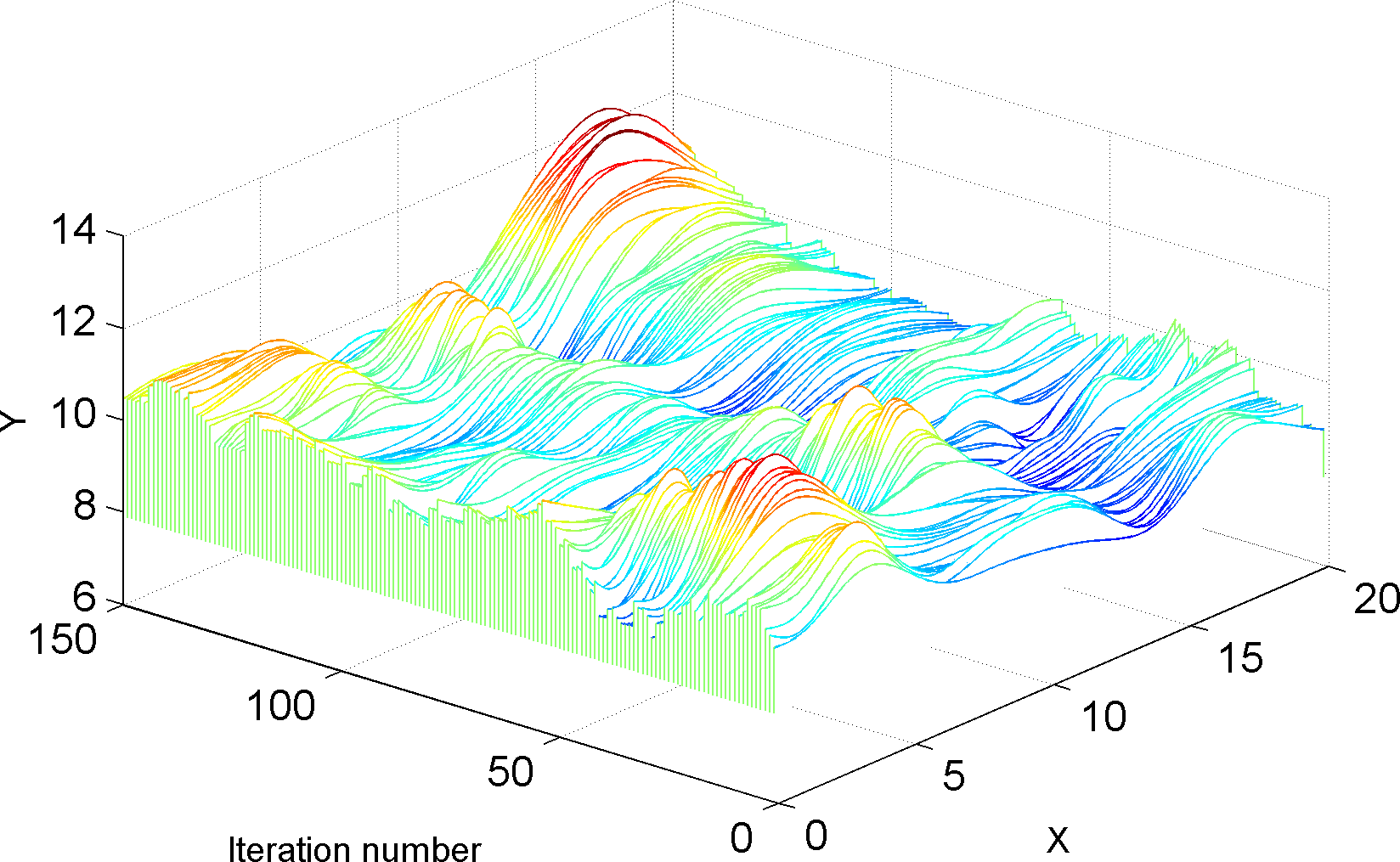