Table of Contents
tomography example This section contains information about how to use and control SIPPI, which requires one to
-
Define the prior model, in form of the prior data structure
-
Define the forward model, in form of the forward data structure, and the sippi_forward.m m-file
-
Define the data and noise model, in form of the prior data structure
[For examples of how to apply SIPPI for different problems, see the section with examples].
A priori information is defined by the prior Matlab structure. Any number of different types of a priori models can be defined. For example a 1D uniform prior can be defined in prior{1}, and 2D Gaussian prior can be defined in prior{2}.
Once a prior data structure has been defined (see examples below), a realization from the prior model can be generated using
m=sippi_prior(prior);
The realization from the prior can be visualized using
sippi_plot_prior(prior,m);
A sample (many realizations) from the prior can be visualized using
m=sippi_plot_prior_sample(prior);
All a priori model types in SIPPI allow to generate a new model in the vicinity of a current model using
[m_new,prior]=sippi_prior(prior,m);
in such a way that the prior model will be sampled if the process is repeated (see Sequential Gibbs Sampling).
Six types of a priori models are available, and can be selected by setting the type
in the prior structure using e.q.
prior{1}.type='gaussian'.
The UNIFORM type prior specifies an uncorrelated ND uniform model.
The GAUSSIAN type prior specifies a 1D generalized Gaussian model.
The FFTMA type prior specifies a 1D-3D Gaussian type a priori model based on the FFT Moving Average method, which is very efficient for unconditional sampling, and for defining a prior Gaussian model with variable/uncertain mean, variance, ranges, and rotation.
The CHOLESKY type prior specifies a 1D-3D Gaussian type a priori model based on Cholesky decomposition of the covariance model,
The VISIM type prior model specifies 1D-3D Gaussian models, utilizing both sequential Gaussian simulation (SGSIM) and direct sequential simulation (DSSIM) that can be conditioned to data of both point- and volume support and linear average data.
The PLURIGAUSSIAN type prior model specifies 1D-3D pluriGaussian. It is a type if truncated Gaussian model that can be used for efficient simulation of categorical values.
The MPS type prior model specifies a 1D-3D multiple-point-based statistical prior model, based on the MPSlib(C++) C++ library. Simulation types includes SNESIM (based on a search tree or list), ENESIM, and GENESIM (generalized ENESIM).
The SNESIM type prior model specifies a 1D-3D multiple-point-based statistical prior model based on the SNESIM code from Stanford/SCRF.
The SNESIM_STD is similar to the 'SNESIM' type prior, but is based on SGEMS.
The following section documents the properties of each type of prior model.
Examples of using different types of prior models or combining prior models can be found in the examples section.
A uniform prior model can be specified using the 'uniform' type prior model
prior{1}.type='uniform';
The only parameters needed are the minimum (min) and maximum (max) values. A 1D uniform distribution between -1 and 1 can be specified as
prior{1}.type='uniform';
prior{1}.min=-1;
prior{1}.max=1;
By setting the x, y, and z parameter, a higher order prior (uncorrelated) can be set. For example 3 independent model parameters with a uniform prior distribution between 20 and 50, can be defined as
prior{1}.type='uniform';
prior{1}.x=[1 2 3];
prior{1}.min=20;
prior{1}.max=50;
Note that using the 'uniform' type priori model, is slightly more computational efficient than using a 'gaussian' type prior model with a high norm.
A 1D generalized Gaussian prior model can be specified using the 'gaussian' type prior model
prior{1}.type='gaussian';
A simple 1D Gaussian distribution with mean 10, and standard deviation 2, can be specified using
ip=1;
prior{ip}.type='gaussian';
prior{ip}.m0=10;
prior{ip}.std=2;
The norm of a generalized Gaussian can be set using the 'norm' field. A generalized 1D Gaussian with mean 10, standard deviation of 2, and a norm of 70, can be specified using (The norm is equivalent to the beta factor referenced in Wikipedia:Generalized_normal_distribution)
ip=2;
prior{ip}.type='gaussian';
prior{ip}.m0=10;
prior{ip}.std=2;
prior{ip}.norm=70;
A 1D distribution with an arbitrary shape can be defined by setting d_target, which must contain a sample of the distribution that one would like to replicate. For example, to generate a sample from a non-symmetric bimodal distribution, one can use e.g.
% Create target distribution
N=10000;
prob_chan=0.3;
d1=randn(1,ceil(N*(1-prob_chan)))*.5+8.5;
d2=randn(1,ceil(N*(prob_chan)))*.5+11.5;
d_target=[d1(:);d2(:)];

% set the target distribution
ip=3;
prior{ip}.type='gaussian';
prior{ip}.d_target=d_target;
The following figure shows the 1D histogram of a sample, consisting of 8000 realizations, generated using
sippi_plot_prior_sample(prior,1:ip,8000);
 |
The FFT moving average method provides an efficient approach for computing unconditional realizations of a Gaussian random field.
The mean and the covariance model must be specified in the m0 and Cm fields. The format for describing the covariance model follows 'gstat' notation, and is described in more details in the mGstat manual.
A 2D covariance model with mean 10, and a Spherical type covariance model can be defined in a 101x101 size grid (1 unit (e.g., meters) between the cells) using
im=1;
prior{im}.type='FFTMA';
prior{im}.x=[0:1:100];
prior{im}.y=[0:1:100];
prior{im}.m0=10;
prior{im}.Cm='1 Sph(10)';
 |
Optionally one can translate the output of the Gaussian simulation into an arbitrarily shaped 'target' distribution, using normal score transformation. Note that this transformation will ensure a certain 1D distribution of the model parameters to be reproduced, but will alter the assumed covariance model such that the properties of covariance model are not necessarily reproduced. To ensure that both the covariance model properties and the 1D distribution are reproduced, make use of the VISIM type prior model instead because it utilizes direct sequential simulation.
im=1;
prior{im}.type='FFTMA';
prior{im}.x=[0:1:100];
prior{im}.y=[0:1:100];
prior{im}.Cm='1 Sph(10)';

% Create target distribution
N=10000;
prob_chan=0.5;
d1=randn(1,ceil(N*(1-prob_chan)))*.5+8.5;
d2=randn(1,ceil(N*(prob_chan)))*.5+11.5;
d_target=[d1(:);d2(:)];
prior{im}.d_target=d_target;
prior{im}.m0=0; % to make sure no trend model is assumed.
Alternatively, the normal score transformation can be defined manually such that the tail behavior can be controlled:
N=10000;
prob_chan=0.5;
d1=randn(1,ceil(N*(1-prob_chan)))*.5+8.5;
d2=randn(1,ceil(N*(prob_chan)))*.5+11.5;
d_target=[d1(:);d2(:)];
[d_nscore,o_nscore]=nscore(d_target,1,1,min(d_target),max(d_target),0);
prior{im}.o_nscore=o_nscore;
 |
The FFTMA method also allows treating the parameters defining the Gaussian model, such as the mean, variance, ranges and angles of rotation as a priori model parameters (that can be inferred as part of inversion, see e.g. an example).
First a prior type defining the Gaussian model must be defined (exactly as listed above):
im=im+1;
prior{im}.type='FFTMA';
prior{im}.x=[0:.1:10]; % X array
prior{im}.y=[0:.1:20]; % Y array
prior{im}.m0=10;
prior{im}.Cm='1 Sph(10,90,.25)';
Now, all parameter such as the mean, variance, ranges and angles of rotations, can be randomized by defining a 1D a priori model type ('uniform' or 'gaussian'), and with a specific 'name' indicating the parameter (see this example for a complete list of names), and by assigning the prior_master field that points the prior model id for which the parameters should randomized.
For example the range along the direction of maximum continuty can be randomized by defining a prior entry named 'range_1', and settting the prior_master to point to the prior with id 1:
im=2;
prior{im}.type='uniform';
prior{im}.name='range_1';
prior{im}.min=2;
prior{im}.max=14;
prior{im}.prior_master=1;
I this case the range is randomized following a uniform distribution U[2,14].
Likewise, the first angle of rotation can be randomized using for example
im=3;
prior{im}.type='gaussian';
prior{im}.name='ang_1';
prior{im}.m0=90;
prior{im}.std=10;
prior{im}.prior_master=1;
A sample from such a prior type model will thus show variability also in the range and angle of rotation, as seen here
 |
im=im+1;
prior{im}.type='VISIM';
prior{im}.x=[0:1:100];
prior{im}.y=[0:1:100];
prior{im}.m0=10;
prior{im}.Cm='1 Sph(10)';
 |
As with the FFTMA prior model the VISIM prior can make use of a target distribution. However, if a target distribution is set, the use of the VISIM prior model will utilize direct sequential simulation, which will ensure both histogram and covariance reproduction.
Using a target distribution together with the VISIM prior model is similar to that for the FFTMA prior model. Simply the type has to be changed from FFTMA to VISIM:
clear all;close all;
im=1;
prior{im}.type='VISIM';
prior{im}.x=[0:1:40];
prior{im}.y=[0:1:40];
prior{im}.m0=10;
prior{im}.Cm='1 Sph(10)';

% Create target distribution
N=10000;
prob_chan=0.5;
d1=randn(1,ceil(N*(1-prob_chan)))*.5+8.5;
d2=randn(1,ceil(N*(prob_chan)))*.5+11.5;
d_target=[d1(:);d2(:)];
prior{im}.d_target=d_target;
 |
The CHOLESKY type prior utilizes Cholesky decomposition of the covariance in order to generate realizations of a Gaussian random field. The CHOLESKY type prior needs a full description of the covariance model, which will be of size [nxyz*nxyz*nxyz], unlike using the FFTMA type prior model that only needs a specification of an isotropic covariance models of size [1,nxyz]. Hence, the CHOLESKY type prior is much more demanding on memory, and CPU. However, the CHOLESKY type prior can be used to sample from any covariance model, also non-stationary covariance model.
The CHOLESKY model is can be defined almost identically to the FFTMA type prior model. As an example:
im=1;
prior{im}.type='CHOLESKY';
prior{im}.x=[0:2:100];
prior{im}.y=[0:2:100];
prior{im}.m0=10;
prior{im}.Cm='1 Sph(10)';
 |
the use of d_target to specify target distributions is also possible, using the same style as for the FFTMA type prior.
Be warned that the 'cholesky' type prior model is much more memory demanding than the 'fftma' and 'visim' type prior models, as a full nxyz*nxyz covariance model needs to setup (and inverted). Thus, the 'cholesky' type prior is mostly applicable when the number of model parameters (nx*ny*nx) is small.
Plurigaussian simulation is a type og truncated Gaussian simulation. It works by generating a number of realizations of Gassuan models, each with a sepcific choice of covariance model. Using a transformation map, the Gaussian realizations are then converted into disrete units.
A simple example using 1 Gaussian realization, one must specify one covariance model one plurigaussian transformation map through the two fields prior{1}.pg_prior{1}.Cm(or Cm) and prior{1}.pg_map.
The covariance model is defined as for any other Gaussian based models, and can include anisotropy. In general, the variance (sill) should be 1. Unless set othwerwise, the mean is assumed to be zero.
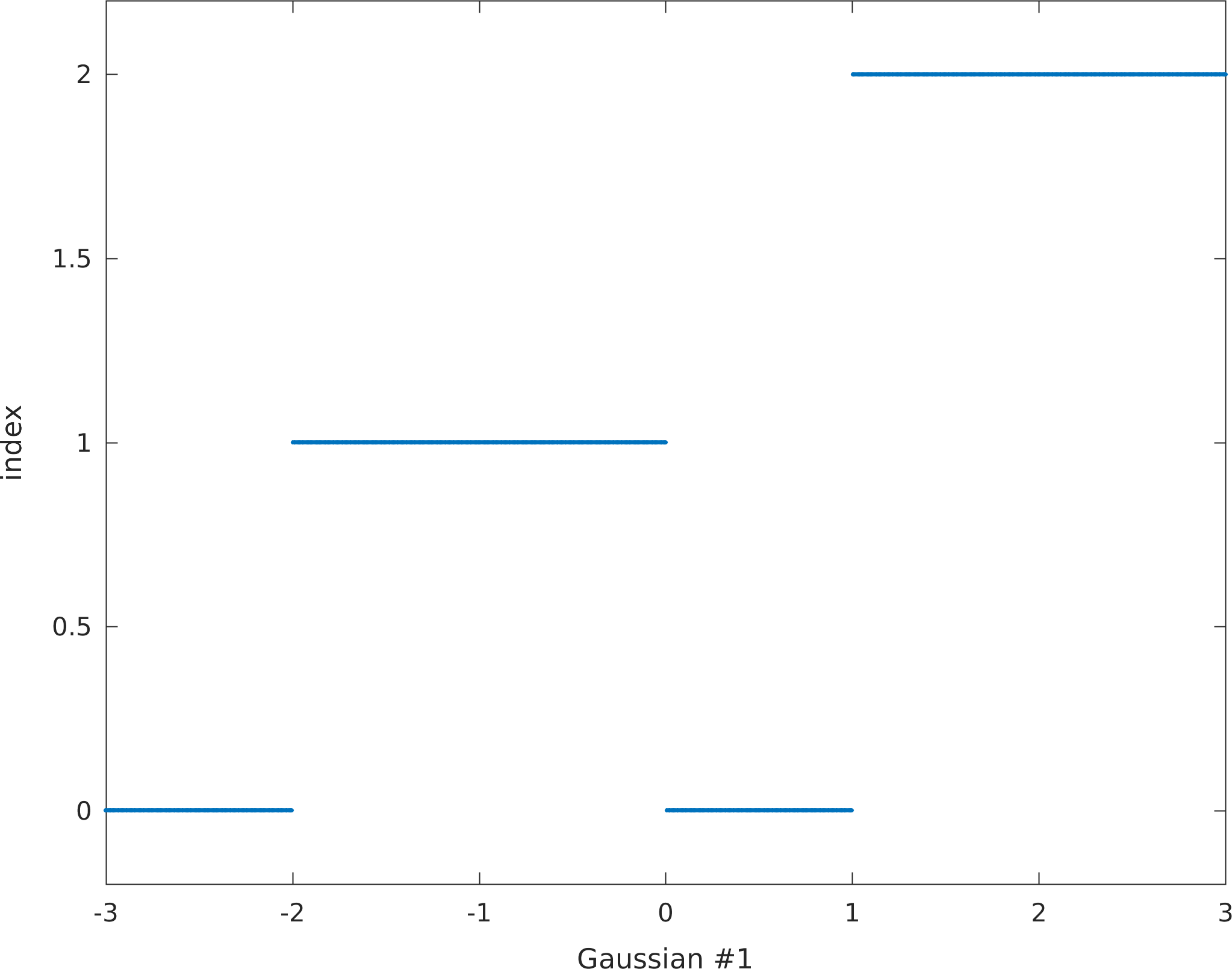
The values in the transformation map is implicitly assumed to define boundaries along a linear scale from -3 to 3. As there are 7 entries (see below) in the transformation map, each number in the transformation map corresponds to [-3,-2,-1,0,1,2,3] respectively. The figure below show what unit id's any Gaussian realized value will be transformed to.
im=im+1;
prior{im}.name='Plurigaussian'; % [optional] specifies name to prior
prior{im}.type='plurigaussian';                % the type of a priori model
prior{im}.x=[0:1:100];                 % specifies the scales of the 1st (X) dimension
prior{im}.y=[10:1:90];                 % specifies the scales of the 2nd (Y) dimension
prior{im}.Cm='1 Gau(10)'; % or next line
prior{im}.pg_prior{1}.Cm=' 1 Gau(10)';
prior{im}.pg_map=[0 0  1 1 0  2 2];
[m,prior]=sippi_prior(prior);          % generate a realization from the prior model
sippi_plot_prior_sample(prior,im,5)
print_mul('prior_example_2d_plurigaussian_1')
figure;
pg_plot(prior{im}.pg_map,prior{im}.pg_limits);
colormap(sippi_colormap);
print_mul('prior_example_2d_plurigaussian_1_pgmap')
 |
 |
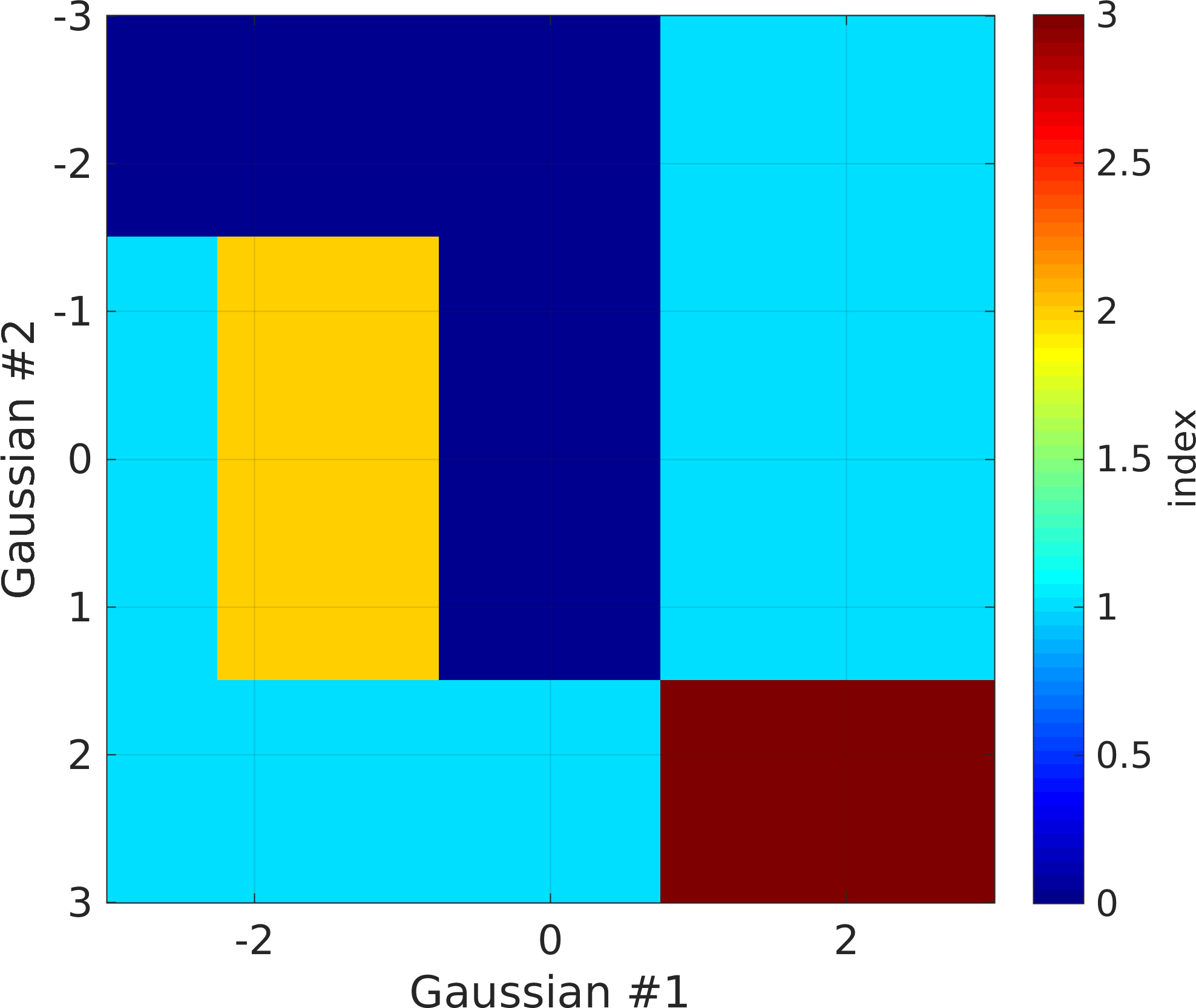
Plurigaussian truncation can be based on more than one Gaussian realization, In the example below, two Gaussian realization are used, and therefore a transformation map needs to be defined. Each dimension of the transformation map corresponds to values of the Gaussian realization between -3 and 3. The transformation maps is visualized below.
im=1;
prior{im}.name='Plurigaussian'; % [optional] specifies name to prior
prior{im}.type='plurigaussian';                % the type of a priori model
prior{im}.x=[0:1:100];                 % specifies the scales of the 1st (X) dimension
prior{im}.y=[10:1:90];                 % specifies the scales of the 2nd (Y) dimension
prior{im}.pg_prior{1}.Cm=' 1 Gau(10)';
prior{im}.pg_prior{2}.Cm=' 1 Sph(10,35,.4)';
prior{im}.pg_map=[0 0 0 1 1; 1 2 0 1 1; 1 1 1 3 3];
[m,prior]=sippi_prior(prior);          % generate a realization from the prior model
sippi_plot_prior_sample(prior,im,5)
print_mul('prior_example_2d_plurigaussian_2')

figure;
pg_plot(prior{im}.pg_map,prior{im}.pg_limits);
set(gca,'FontSize',16)
colormap(sippi_colormap);
print_mul('prior_example_2d_plurigaussian_2_pgmap')
 |
 |
The 'MPS' type prior make use of the MPSlib(C++) library for mulitple-point based simulation. For compilation and installation help see Install SIPPI. MPSlib(C++) implements the SNESIM (using both a search tree and a list to stor conditional statistics), and the generalized ENESIM algoritm. The type of multiple-point algorithm is define in the method field.
To use the MPS type prior at least the type, dimension, as well as a training image must be provided:
ip=1;
prior{ip}.type='mps';
prior{ip}.x=1:1:80;
prior{ip}.y=1:1:80;
A trainin imag emust be set in the 'ti' field, as 1D, 2D, or 3D matrix. If not set, the classical training image from Strebelle is used, equivalent to:
prior{ip}.ti=channels;
More examples of traning images are located in the 'mGstat/ti' folder.
MPSlib(C++) provides three different simulation aglrithms, which canbe chosen in the 'method' field as:
prior{ip}.method='mps_snesim_tree';
prior{ip}.method='mps_snesim_list';
prior{ip}.method='mps_genesim';
'mps_snesim_tree' is the simulation method selected by default if it is not specified.
All options for the MPS type simulation algorithm are be available in the prior{ip}.MPS data structure.
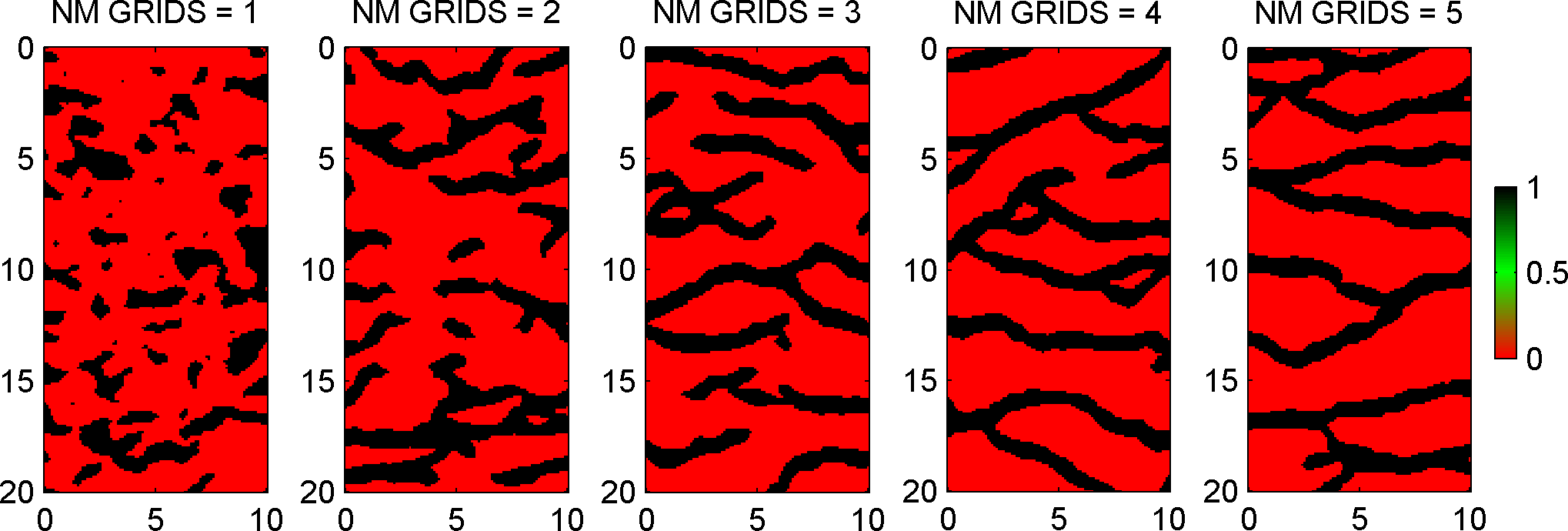
For example, to set the number of used multiple grids, set the MPS.n_multiple_grids as
ip=1;
prior{ip}.type='mps';
prior{ip}.method='mps_snesim';
prior{ip}.x=0:.1:10;
prior{ip}.y=0:.1:20;
[m,prior]=sippi_prior(prior);
i=0;
for n_mul_grids=[0:1:4];
    prior{ip}.MPS.rseed=1;
    prior{ip}.MPS.n_multiple_grids=n_mul_grids;
    [m,prior]=sippi_prior(prior);
    i=i+1;subplot(1,5,i);
    imagesc(prior{1}.x,prior{1}.y,m{1});axis image
    title(sprintf('NMG = %d',n_mul_grids));
end
More details on the use of MPSlib(C++) can be found in the SoftwareX manuscript that describes MPSlib(C++).
The 'SNESIM' type prior model utilizes the SNESIM algorithm, as implemented in Fortran available at Stanford/SCRF.
By default a training image (channel structures) from Sebastian Strebelle's PhD theses is used (if no training image is specified). A simple 2D type SNESIM prior model can be defined using the following code:
ip=1;
prior{ip}.type='SNESIM';
prior{ip}.x=[0:.1:10]; % X array
prior{ip}.y=[0:.1:20]; % Y array
and 5 realizations from this prior can be visualized using
for i=1:5;
    m=sippi_prior(prior);
    subplot(1,5,i);
    imagesc(prior{1}.x,prior{1}.y,m{1});axis image
end
 |
Note that the training image is always assumed to have the same units as the prior model, so in this case each pixel in the training image is assumed to be separated by a distance '0.1'.
Optionally 'scaling' and 'rotation' of the training image can be set. To scale the training image by 0.7 (i.e., structures will appear 30% smaller) and rotate the training 30 degrees from north use
ip=1;
prior{ip}.type='SNESIM';
prior{ip}.x=[0:.1:10]; % X array
prior{ip}.y=[0:.1:20]; % Y array
prior{ip}.scaling=.7;
prior{ip}.rotation=30;
 |
A custom training image can be set using the ti field, which must be either a 2D or 3D matrix.
% create TI from image
EXAMPLE EXAMPLE

% setup the prior
ip=1;
prior{ip}.type='SNESIM';
prior{ip}.x=[0:.1:10]; % X array
prior{ip}.y=[0:.1:20]; % Y array
prior{ip}.ti=ti;
Note that the training image MUST consist of integer index values starting from 0 (i.e. '0', '1', '2', ...).
If the prior structure is returned from sippi_prior using
[m,prior]=sippi_prior(prior);
then an XML structure prior{1}.S.XML will be available. This allows a complete customization of all settings available in SGeMS. For example, the different realizations, using 1, 2, and 3 multiple grids can be obtained using
ip=1;
prior{ip}.type='SNESIM';
prior{ip}.x=[0:.1:10]; % X array
prior{ip}.y=[0:.1:20]; % Y array
[m,prior]=sippi_prior(prior);
for i=1:5;
    prior{ip}.S.XML.parameters.Nb_Multigrids_ADVANCED.value=i;
	subplot(1,3,5);
    imagesc(prior{1}.x,prior{1}.y,m{1});axis image
end
 |
The 'SNESIM' type prior model utilizes the SNESIM algorithm, as implemented in SGeMS. It can be called using the options as sippi_prior_snesim.
Once the prior data structure has been defined/modified, a sample from the prior distribution can be generated using
m=sippi_prior(prior);
'm' is a Matlab data structure of the same size as the 'prior' data structure. Thus, if two prior distributions have been defined in 'prior{1}' and 'prior{2}', then 'm{1}' will hold a realization of 'prior{1}', and 'm{2}' will hold a realization of 'prior{2}'.
Each time 'm=sippi_prior(prior)' is called, a new independent realization of the prior will be generated.
All the available types of prior models allow perturbing one realization of a prior into a new realization of the prior, where the degree of perturbation can be controlled (from a new independent realization to a very small change).
This means that a random walk, with an arbitrary 'step-length' can be performed for any of the a priori types available in SIPPI
For the a priori types 'FFTMA', 'VISIM', 'CHOLESKY', 'SISIM', 'SNESIM', sequential Gibbs sampling [HCM12] is applied. Sequential Gibbs is in essence a type of conditional re-simulation. From a current realization of a prior model, a number of model parameters are discarded and treated as unknown. The unknown model parameters are then re-simulated conditional to the known model parameters.
In order to generate a new realization 'm2' in the vicinity of the realization 'm1' use
[m1,prior]=sippi_prior(prior);
[m2,prior]=sippi_prior(prior,m1);
If this process is iterated, then a random walk in the space of a priori acceptable models will be perform. Moreover, the collection of realization obtained in this way will represent a sample from prior distribution.
Note that in order to use sequential Gibbs sampling prior must be given both as an input variable, and as an (possibly update) output variable.
All properties related to sequential Gibbs sampling can be set in the 'seq_gibbs' structure (which will be avaiable the first time sippi_prior is called, or if sippi_prior_init is called), for the individual prior models.
The step-length (i.e. the degree of perturbation) is determined by the prior{m}.seq_gibbs.step parameter.
For the 'uniform' and 'gaussian' type a priori models a step-length closer to 0 zeros imples a 'shorter' step, while a step-length close to 1, implies a 'longer' step-length. A step length of 1, will generate a new independent realization of the prior, while a step length of 0, will return the same realization of the prior
prior{m}.seq_gibbs.step=.1;
[m2,prior]=sippi_prior(prior,m1);
For the 'FFTMA', 'VISIM', 'CHOLESKY', 'SISIM', and 'SNESIM' type a priori models two types (defined in the prior{m}.seq_gibbs.type variable).
The default 'type' is 2, defined as
prior{m}.seq_gibbs.step=1;
prior{m}.seq_gibbs.type=2;
where the step length defines the percentage of the of model parameters (selected at random) defined in prior{im} is conditionally re-sampled. Thus, a step-length closer to 0 zeros imples a 'shorter' step, while a step-length close to 1, implies a 'longer' step-length.
If prior{m}.seq_gibbs.step=1, then prior{m}.seq_gibbs.step defines the size of a square rectangle/cube which is to be conditionally re-simulated using sequential Gibbs sampling.