In the following a simple 2D Gaussian a priori model is defined, and SIPPI is used to sample the corresponding a posteriori distribution. (An example script is avalable at examples/case_tomography/sippi_AM13_metropolis_gaussian.m).
Initially we load the travel time data obtained at Arrenæs (See Arrenæs Data for more information)
D=load('AM13_data.mat');
This allow us to setup a SIPPI data structure defining the observed data as well as the associated model of uncertainty
%% SETUP DATA
id=1;
data{id}.d_obs=D.d_obs;
data{id}.d_std=D.d_std;
data{id}.dt=0; % Mean modelization error
data{id}.Ct=1; % Covariance describing modelization error
In the above example we define a Gaussian modelization error, N(dt,Ct). We do this because we will make use of a forward model, the eikonal solver, that we know will systematically provide faster travel times than can be obtained from the earth. In reality the wave travelling between bore holes never has infinitely high frequency as assumed by using the eikonal solver. The eikonal solver provides the fast travel time along a ray connecting the source and receiver. Therefore we introduce a modelization error, that will allow all the travel times to be biased with the same travel time.
The a priori model is defined using the prior data structure. Here a 2D Gaussian type a priori model in a 7x13 m grid (grid cell size .25m) using the FFTMA type a priori model. The a priori mean is 0.145 m/ns, and the covariance function a Spherical type covariance model with a range of 6m, and a sill(variance) of 0.0003 m^2/ns^2.
%% SETUP PRIOR
im=1;
prior{im}.type='FFTMA';
prior{im}.m0=0.145;
prior{im}.Va='.0003 Sph(6)';
prior{im}.x=[-1:.15:6];
prior{im}.y=[0:.15:13];
One could make used of the VISIM type priori model simply by substituting 'FFTMA' with 'VISIM' above.
'sippi_forward_traveltime' require that the location of the sources an receivers are provided in 'forward' structure using the 'sources' and 'receivers' field names.
D=load('AM13_data.mat');
forward.forward_function='sippi_forward_traveltime';
forward.sources=D.S;
forward.receivers=D.R;
forward.type='eikonal';
Here the eikonal solution is chosen to solve the forward problem. See more detail about solving the forward problem related to cross hole first arrival travel time computation here.
As the
prior,
data, and
forward have been defined, one can in principle initiate an inversion. However, it is advised to perform a few test before applying the inversion.
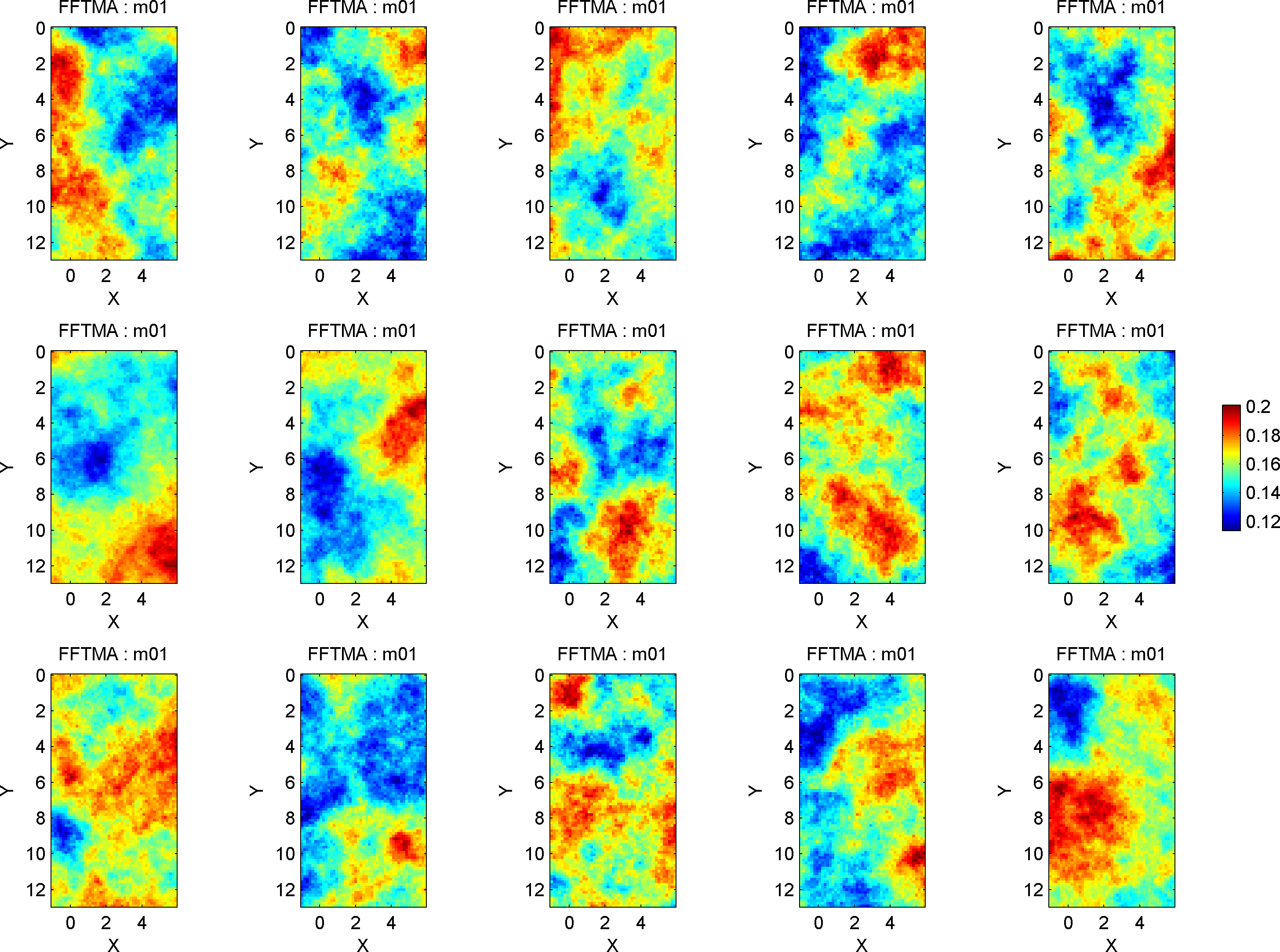
First, one should check that independent realization of the prior model resemble the a priori knowledge. A sample from the prior model can be generated and visualized calling sippi_plot_prior_sample:
sippi_plot_prior_sample(prior);
which provides the following figure
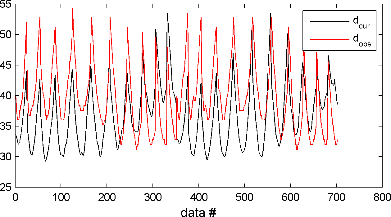
The one can check that the forward solver, and the computation of the likelihood wors as expected using
% generate a realization from the prior
m=sippi_prior(prior);
% Compute the forward response related to the realization of the prior model generated above
[d]=sippi_forward(m,forward,prior,data);
% Compute the likelihood
[logL,L,data]=sippi_likelihood(d,data);
% plot the forward response and compare it to the observed data
sippi_plot_data(d,data);
which produce a figure similar to
The extended Metropolis sampler can now be run using sippi_metropolis.
options=sippi_metropolis(data,prior,forward);
In practice the user will have to set a few options, controlling the behavior of the algorithm. In the following example the number of iterations is set to 500000; the current model is saved to disc for every 500 iterations; the log-likelihood and current model is shown for every 1000 iterations:
options.mcmc.nite=500000; % optional, default:nite=30000
options.mcmc.i_sample=500; % optional, default:i_sample=500;
options.mcmc.i_plot=1000; % optional, default:i_plot=50;
options=sippi_metropolis(data,prior,forward,options);
By default no annealing schedule is used. By default the 'step'-length for sequential Gibbs sampling is adjusted (to obtain an average acceptance ratio of 30%) for every 50 iterations until iteration number 1000.
An output folder will be generated with a filename formatted using 'YYYYMMDD-HHMM', followed by a automatic description. In the above case the output folder could be name '20140701_1450_sippi_metropolis_eikonal'.
The actual folder name is return in options.txt.
One can define a description for the folder name by setting options.txt before running sippi_metropolis.
The folder contains one mat file, with the same name as the folder name, and N ASCII files (where N=length(prior); one for each a priori type) which contains the models saved to disc. They also have the same name as the folder name, appended with '_m1.asc', '_m2.asc', and so forth.
The function sippi_plot_posterior can be called when sippi_metropolis (or sippi_rejection) and will plot the progress of the log-likelihood curve, a sample of the posterior, data response from a sample of the posterior, and (if applicable) 1D and 2D marginal posterior distributions.
Located in the output folder of the inversion use
sippi_plot_posterior;
If the location of the folder with the output is known (such as options.txt) one can call
sippi_plot_posterior(options.txt)

