Firs the Jura data is loaded.

% jura_covariance_inference
%
% Example of inferring properties of a Gaussian model from point data
%

%% LOAD THE JURA DATA
clear all;close all
[d_prediction,d_transect,d_validation,h_prediction,h_transect,h_validation,x,y,pos_est]=jura;
ix=1;
iy=2;
id=6;

% get the position of the data
pos_known=[d_prediction(:,[ix iy])];  

% perform normal score transformation of tha original data
[d,o_nscore]=nscore(d_prediction(:,id));
h_tit=h_prediction{id};

First a SIPPI 'prior' data structure is setup do infer covariance model parameters for a 2D an-isotropic covariance model. That is, the range_1, range_2, ang_1, and nugget_fraction are defined using

im=0;
% A close to uniform distribution of the range, U[0;3].
im=im+1;
prior{im}.type='uniform';
prior{im}.name='range_1';
prior{im}.min=0;
prior{im}.max=3;

im=im+1;
prior{im}.type='uniform';
prior{im}.name='range_2';
prior{im}.min=0;
prior{im}.max=3;

im=im+1;
prior{im}.type='uniform';
prior{im}.name='ang_1';
prior{im}.min=0;
prior{im}.max=90;

im=im+1;
prior{im}.type='uniform';
prior{im}.name='nugget_fraction';
prior{im}.min=0;
prior{im}.max=1;

Thus the a priori information consists of uniform distributions of ranges between 0 and 3, rotation between 0 and 90, and a nugget fraction between 0 and 1 is.

Then the data structure is set up, using the Jura data selected above, while assuming a Gaussian measurement uncertainty with a standard deviation of 0.1 times the standard deviation of the data:

%% DATA
data{1}.d_obs=d; % observed data
data{1}.d_std=0.1*std(d);.4; % uncertainty of observed data (in form of standard deviation of the noise)

Finally the forward structure is setup such that sippi_forward_covariance_inference allow inference of covariance model parameters.

In the forward structure the location of the point data needs to be given in the pos_known field, and the initial mean and covariance needs to be set. Also, the name of the forward function used (in this case sippi_forward_covariance_inference) must be set. Use e.g.:

%% FORWARD
forward.forward_function='sippi_forward_covariance_inference';
forward.point_support=1;
forward.pos_known=pos_known;

% initial choice of N(m0,Cm), mean and sill are 0, and 1, due
% due to normal score
forward.m0=mean(d);
forward.Cm=sprintf('%3.1f Sph(2)',var(d));

Now, SIPPI is set up for inference of covariance model parameters. Use for example the Metropolis sampler to sample the a posterior distribution over the covariance model parameters using:

options.mcmc.nite=100000;
options.mcmc.i_plot=1000;
options.mcmc.i_sample=25;
options.txt=name;
[options,data,prior,forward,m_current]=sippi_metropolis(data,prior,forward,options)

sippi_plot_prior(options.txt);
sippi_plot_posterior(options.txt);

Sampling the posterior provides the following 2D marginal distributions

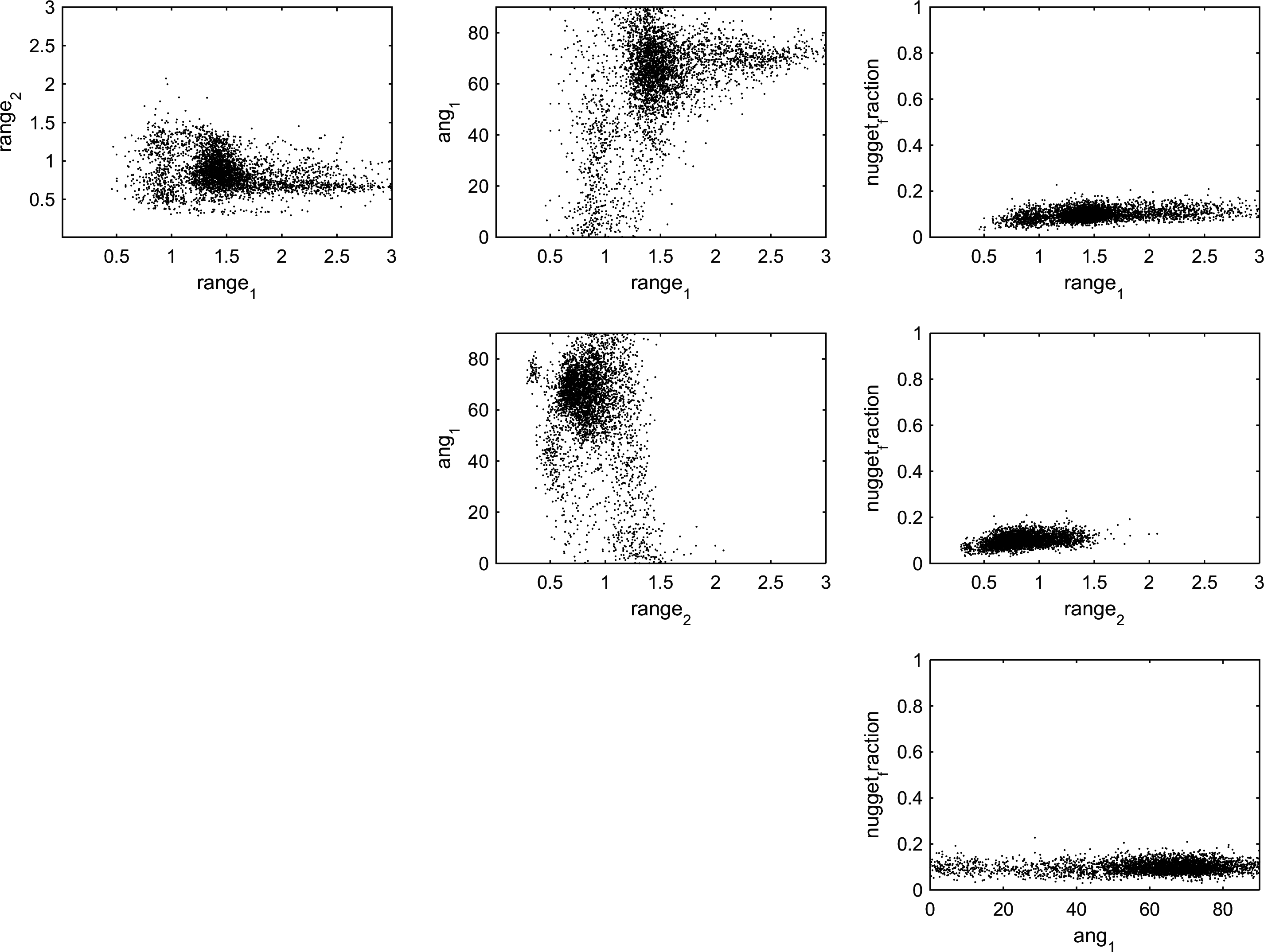Note how several areas of high density scatter points (i.e. areas with high posterior probability) can be found.