[A Matlab script for the following example is avalable at examples/case_tomography/sippi_AM13_metropolis_bimodal.m.]

The GAUSSIAN and FFTMAa prior types implicitly assume a normal distribution of the model parameter.

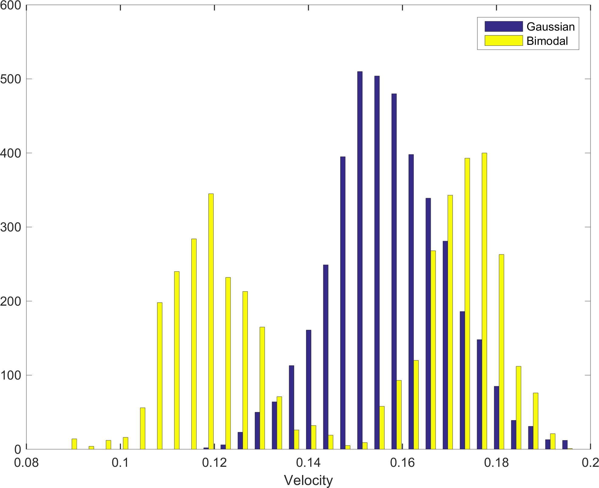
It is however possible to change the Gaussian distribution to any shaped distribution, using a normal score transform. Note that when this is done the given semivariogram model for the FFTMA a priori model will not be reproduced. If this is a concern, then the VISIM type a priori model should be used.

The data and forward structures is identical to the one described in the previous example.

%% Load the travel time data set from ARRENAES
clear all;close all
D=load('AM13_data.mat');
options.txt='AM13';

%% SETUP DATA
id=1;
data{id}.d_obs=D.d_obs;
data{id}.d_std=D.d_std;
data{id}.Ct=D.Ct+1; % Covariance describing modeling error

% SETUP THE FORWARD MODEL USED IN INVERSION
forward.forward_function='sippi_forward_traveltime';
forward.sources=D.S;
forward.receivers=D.R;
forward.type='fat';forward.linear=1;forward.freq=0.1;

The desired distribution (the 'target' distribution) must be provided as a sample of the target distribution, in the data{id}.d_target distribution.

%% SETUP PRIOR
im=1;
prior{im}.type='FFTMA';
prior{im}.name='Velocity (m/ns)';
prior{im}.m0=0.145;
prior{im}.Va='.0003 Sph(6)';
dx=0.15;
prior{im}.x=[-1:dx:6];
prior{im}.y=[0:dx:13];
prior{im}.cax=[.1 .18];

% SET TARGET
N=1000;
prob_chan=0.5;
dd=.014*2;
d1=randn(1,ceil(N*(1-prob_chan)))*.01+0.145-dd;  %0.1125;
d2=randn(1,ceil(N*(prob_chan)))*.01+0.145+dd; %0.155;
d_target=[d1(:);d2(:)];
prior{im}.d_target=d_target;

5 realizations from the corresponding a priori model looks like

Figure Figure 4.6, “Distribution of one realization using a Gaussian Bimodal target distribution” compares the distribution from one realization of both prior models considered above.

As for the examples above, the a posteriori distribution can be samples using e.g.

options.mcmc.nite=500000; % optional, default:nite=30000
options.mcmc.i_sample=500; % optional, default:i_sample=500;
options.mcmc.i_plot=1000; % optional, default:i_plot=50;
options=sippi_metropolis(data,prior,forward,options);

% plot posterior statistics
sippi_plot_posterior(options.txt);